Convolution, Cross-Correlation and Gaussian

In this post, we will continue to learn more about low-level computer vision which we’ve started in last post. After reading this post you will learn Convolution as well as literally most of the computer vision because it appears somehow in all functions that we will use in the CV. Let’s get started.

Convolution and Cross-Correlation

Let’s have a look at difinition of Discrete Convolution and cross-correlation in mathematics:

1) Convolution:

$(f * g)[n] = \sum_{m=-\infty}^\infty f[m]g[n-m]$

2) Cross-Correlation:

$(f * g)[n] = \sum_{m=-\infty}^\infty f[m]g[n+m]$

As we can see in convolution the function g, first, should be mirrored and then shifted step by step and finally, in each step, it will be multiplied by the function f and the results will be summed up. The only difference between Convolution and Cross-Correlation (Correlation) is that in Cross-Correlation there is no mirroring in function g.

But before continue we need to define kernel. A kernel is just a matrix and we will use them to do some cool things such as sharpening, blurring, edge detection, etc. The value that we use for each cell in a kernel determines its functionality.

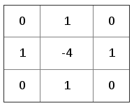
In Digital Image Processing, sometimes, results of convolution and correlation are the same, hence the kernel is symmetric (like Gaussian, Laplacian, Box Blur, etc.) and so flipping the kernel does not change the result by applying convolution. So, don’t be surprised if people sometimes calculate the correlation and call it convolution. For instance, the following figure, Fig. 1, represents an edge detection kernel and if we flip it to the x-axis (second row which includes the anchor point), the result would be the same kernel and also the result of convolution and correlation would be the same.

Color Spectrum — Fig. 1: Edge Detection Kernel

But which one should be used? We prefer to use convolution because it gives us a nice property which is the associativity. That means, applying Fourier Transformation to the convolution of two functions in Spatial domain is equal to the product of Fourier Transformation of two functions:

$g(t) * h(t) <--> G(\mu).H(\mu)$

$F[g * h] = F[g].F[h]$

By applying cross-correlation in Spatial domain is equal to the product of a function with complex conjugate of the other one:

$g(t) o h(t) <--> G(\mu).H(\mu)^*$

$F[g o h] = F[g].F[h]^*$

Choosing the size and values for the kernel depends on what we want to do with our image and we may talk about it in further articles.

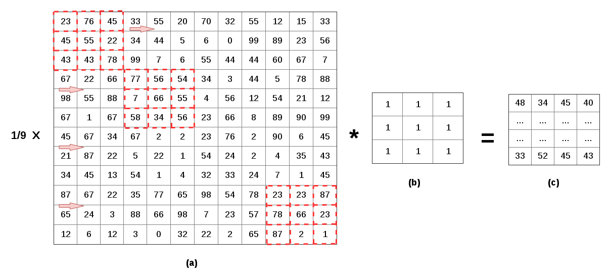
To make things more clear about convolution and cross-correlation, let’s consider an example, say we have a 12×12 image and we want to shrink it to 4×4, as shown in Fig. 2. So each 3×3 pixels (9 pixels) in 12×12 image should be reduced to 1 pixel, to do that we can consider to ways:

1) take the value of the pixel in the center of the 3×3 box and produce the 4×4 image (If there is no center cell in the kernel what we can do is using interpolation to estimate the value for the center cell), using this method results in some artifacts in the new image. 2) take the average of 9-pixel values and put it in the new image.

The second choice produces a better result. The averaging operation is a weighted sum (adding up all of the pixel values and divide it by the number of pixels which here is 9). So for shrinking the original image, we can summarize it in the following steps:

1) Put the kernel in the first patch of the original image and calculate the average and put it in the first pixel of new image 2) Move the kernel to the next patch, 3 pixels further (top-left cell of the kernel should be in forth pixel), and calculate the average. We shift the kernel by 3 pixels to the right/down to shrink the image. The result of the shrinking using convolution or cross-correlation should be the same.

To get some more intuition about that you can take a look at this blog post and also you can find the C++ implementation of what we have discussed so far on my Github Repository.

For doing other things like blurring, sharpening, etc we consider a one-pixel shift for the kernel.

This type of kernel, (b) in Fig.2, is also called “box filter/box blur/averaging”. Box filter is used for smoothing the images by considering a step movement for that. Usually smoothing is used for reducing noises in an image like sensor noise. But the box filter will not give a perfect result if the image contains vertical/horizontal lines (such as trees), because the lines in the resulting image are not clear. To avoid this problem we can use the Gaussian filter.

Gaussian filter (Normal/Gaussian distribution)

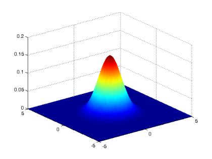
The Gaussian filter can be considered as a low pass filter so that the mean of Gaussian filter defines the center of the bell shape (which is the main frequency that we want to pass) and the standard deviation defines how wide the bell-shaped curve is (the bandwidth of filter), see Fig. 3. Generally, 2D Gaussian filter/distribution will be defined by the following formula:

$G(x,y) = \frac{1}{2\pi\sigma^2}e^{-\frac{x^2+y^2}{2\sigma^2}}$

So if we go closer towards the mean in the filter the pixel values are contributing significantly more to the result.

As we know the image is a spatial discrete/digital matrix, so what we need to do before convolution is approximating (discrete) Gaussian kernel which will be a very large matrix, and consequently, the computation time for calculating convolution will increase, so we need to reduce kernel size. There are different algorithms for approximating the Gaussian kernel and if you are interested in that you can read this article on StackExchange, signal processing.

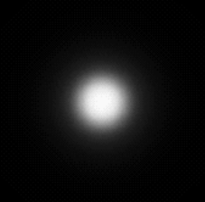
The elements in the center of this Gaussian kernel should have a higher value (white) than elements near to the edge of the kernel (black), so if we plot that it will look something like Fig 4.

Summary and important notes

Generally, there is a problem with kernels and it happens whenever the kernel is near to the edge and corners of the image. To solve this problem there some solutions:

ignore pixels near to corners and edges
create some extra pixels for parts of the kernel which are outside of the original image
duplicate/reflect the value of edges
etc.

Basically, in convolutional operation using weighted sums, we can use two types of kernels:

Kernels in which the sum of elements is one. This kernel sharpens the image and does not have a significant effect on the brightness or darkness of the image.
Kernels in which the sum of elements is zero. This kernel is used for edge detection, because if the color significantly changed, as it happens on edges, the value of that pixel would be multiplied by a large positive number from the kernel. These kernels are like a high pass filter.

Convolution features:

Commutative: A * B = B * A
Distribution over addition: A*(B+C) = A * B + A * C
Associative: A*(B * C) = (A * B) * C
Scalars: x(A*B) = (xA) * B = A * (xB)
2D gaussian is just composition of 1D gaussians, and it is faster to run two 1D convolutions

Most of Computer Vision is based on convolution and the following list is some of the cool things that we can do with convolution:

Sharpening/Blurring the image
Edge detection
Feature detection
Get derivative
Make High resolution
Classification
Detection
Image captioning
etc.

Note that we can apply multiple kernels to the image and get some bunch of different outputs and then we can combine these outputs in some new ways and get some results that are basically on top of understanding the image and that is all neural network is doing. So what neural network (or machine learning in general) is doing is applying a bunch of kernel to the image and then taking the result of that operation and applying more operation on top of that.

Tags:Computer Vision, Convolution, Cross-Correlation, Gaussian filter, low-level Computer Vision, Machine Learning

About The Author

Tech Enthusiast

Convolution and Cross-Correlation

Gaussian filter (Normal/Gaussian distribution)

Summary and important notes

Related Posts

About The Author

Add a Comment